The 4 Stages of MLOps Journey

MLOps is about deploying and maintaining production models. In this blog post, we go through various stages in the journey to MLOps nirvana.

You have worked hard on identifying a problem that can benefit from machine learning. you have spent hours on building the model. You have verified the metrics and double checked the confusion matrices. Things look great. What to do next? You want to get the model live! What’s the best way to get the model into production so that it can be consumed by real users like you and me?

Climbing the MLOps maturity ladder is like hiking on a mountain (Source)

The question is answered by Machine Learning deployments. ML Deployment takes a model and deploys it to, say, a server so that it can be served to a real public. The mechanics of managing deployments is controlled by MLOps. MLOps or Machine Learning Operations is an analogous term derived from DevOps. In DevOps you do everything to get a website running smoothly on servers running either on-prem or on a cloud provider. Likewise, in MLOps you do everything to to get a model running smoothly so that it can be of value to real users.

Let’s take a few examples of real-life ML use-cases to help us understand the different stages of MLOps journey:

1. Transcribing a YouTube video (batch prediction, batch serving)

2. Recommending movies on Netflix (batch prediction, online serving)

3. Recommend best size of a dress based on measurements (online prediction, online serving)

4. Predicting price of an Uber ride (online prediction with Near Real time (NRT) features, online serving)

Note: This blog has an oversimplification of the above systems and real-life systems are going to be much more complex and may not work as described.

To understand the 4 stages of MLOps journey, it’s important to go through the three steps of any machine learning model lifecycle.

Model Training

Model training is at the heart of machine learning and is also a lot of fun! You might take labels of images and train a convolutional neural network to classify images into different categories (classification). Or you might do pricing of Uber rides (regression). Or you might cluster houses in your area into different groups (unsupervised clustering). All of these tasks need some form of training data — and you train a model to learn patterns from the data.

With regards to MLOps discussion, model is a black box that takes in data as features and then outputs a prediction. A simpler to train model may have more complex MLOps needs than a more complex to train model.

Features for model training

In MLOps discussion, features for model training matter quite a lot more than model architecture itself. There are different kind of features that may be available to a model:

1. Batch features: These features may be things like aggregation of movies liked by a user or days since registration. These features are recomputed once say daily or monthly in batch jobs and don’t change very quickly. Batch jobs typically run on Spark clusters if your data is large. These features are pre-computed. These features may need to served online for online model inference via fast-read online features stores or caches (BigTable, MySQL, Redis etc).

2. Near Real Time (NRT) features: These features are more responsive than batch features and are available in “almost” real time. When do we need such features? Say you are predicting price of an Uber ride — you could use static features such as your country or registration date but you also need NRT features such as how many riders are in the area in last 30 min. You are willing to accept a delay or lag of 1 or 2 min. Another example of NRT feature is last 5 posts liked by a user on Instagram. You may have a batch feature such as total number of posts liked by a user, but you may want to supplement it with last 5 posts liked for more near real time signal.

3. Real Time (RT) features: These features are in the request path. Example of such features are device, time of day, location, a person’s measurements for fit etc. These features are only available when the user is making a request and cannot be precomputed.

This distinction will become important in our discussion of MLOps journey.

Model Prediction

Model prediction or inference involves making predictions from actual data or held-out test data. Typically the saved artifacts from the model training step are read in and used to load the model architecture and weights, and features from actual data are used to compute the predictions. These predictions may be returned in JSON format such as:
{"user_id": 14a1sd112325d1e45a, "movie_id": 23b4ab122sdga3ad1v, "similarity": 0.7123} This stage allows the model to infer on features and create a prediction.

Predictions Serving

This stage is the one that determines how’d the predictions actually get into the hands of users/ customers. For some models predictions are served right after model inference (say for predicting price of an Uber ride), but for some models it might make sense to infer first and serve the predictions at another time (movie recommendations on Netflix).

Now let’s use these fundamental concepts to understand the various stages of MLOps.

Stage 1: Batch prediction, batch serving

The example we are taking for the first stage is transcribing of YouTube video.

A video may be uploaded by a user and may enter a queue for processing. A ML model which was trained offline to analyze audio data would be used to parse over the uploaded videos sequentially. The ML Model would output the text of the transcribed video and write it to a storage platform such as S3 or Google Cloud Storage. Pre-computed predictions can then be served for downstream jobs which will consume these in batch. An example of this might be a translation model that’d read from the S3 or GCS bucket and perform conversions to other languages offline.

Simplest stage in ML journey is to save predictions once a day and then read them as needed

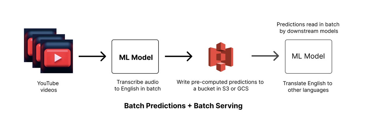
The first ML model is an example of batch prediction and batch serving. Our inference as well as serving of predictions is happening in batch offline. Neither the prediction or its serving is happening on the request path. This is the first stage of our MLOps journey.

As can be seen in the diagram, usually batch prediction and batch serving is meant for other downstream models to consume predictions in batch.

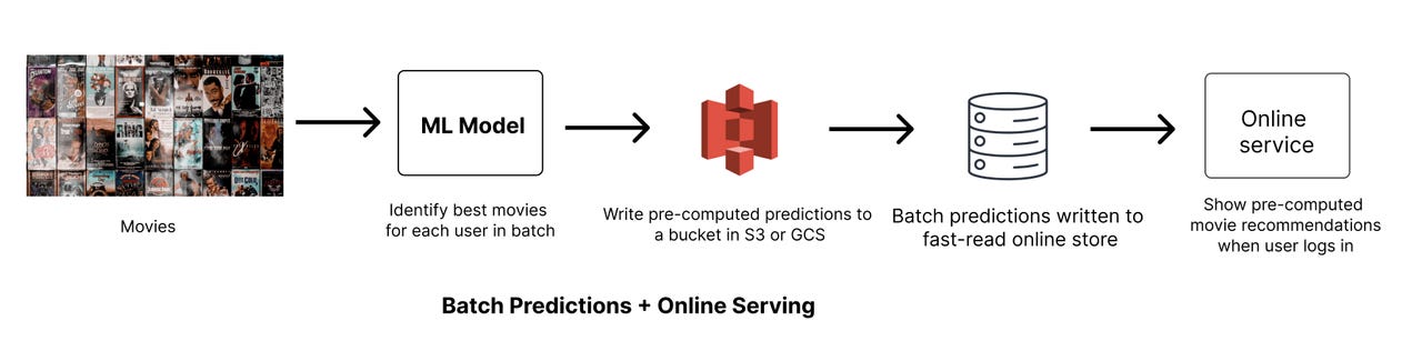
Stage 2: Batch prediction, online serving

Next stage is a continuation of Stage 1. Instead of the downstream model also handling predictions in batch, now it’s a service instead which is serving predictions live to real users -> and your model output is being fed into the online service from a database or cache. An example of such a system is movie recommendations on Netflix.

In both stage 1 and stage 2, recommendations or predictions are generated offline in batch — the key difference is how downstream is consuming these. In the first stage, downstream models read the predictions in batch, but here we need to load the predictions to a fast database or cache for online serving. These read times are fast ranging from ~10ms-100ms.

Next stage is to still do predictions once a day but serve them online using a DB

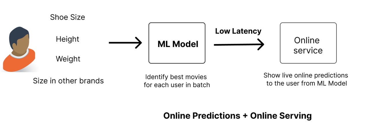
Stage 3: Online prediction, online serving

In this stage we move from batch pre-computed predictions to online predictions. Here we only run model inference at the time of actual online request. The key advantage of this is that we only need to run inference on users active on our platform and do not need to pre-compute predictions for everyone.

The main disadvantage is that we need to maintain a low-latency system to support this use case. These predictions are served online in the request path. An example of such a system is predicting best size of the dress based on measurements. Users are expected to key-in their body measurements and the ML model returns the best size for a dress for different brands.

Why can’t we do online prediction in batch? The reason is that we don’t know the features before-hand. Body measurements are only available when a user logs into (say) Adidas or Nike store and is looking for immediate results on measurements.

ChatGPT is another example where the model has to run live inference on online features.

Diagram of how this stage might look:

This stage involves “live” predictions from user input

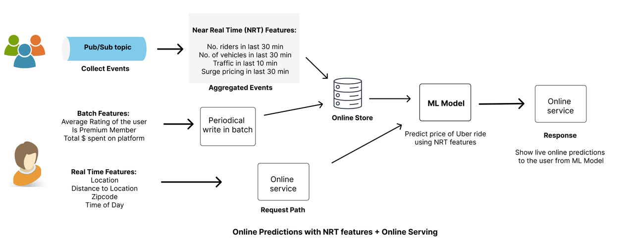
Stage 4: Online prediction with NRT features, online serving

Continuing on, Stage 4 is an extension of Stage 3 as this stage now has NRT or Near Real Time features. Let’s take example of predicting price of an Uber ride.

What are some examples of NRT features for predicting price of an Uber ride?

1. Number of riders in the last 30 min

2. Number of vehicles in the last 30 min

3. Traffic congestion in the last 10 min

4. Surge pricing in the last 30 min

Some Real time (RT) features that can also help the model are

1. Location

2. Distance to destination

3. Time of day

Some batch features that are helpful for this model can be:

1. Average rating of the rider

2. Premium or non-premium member

3. Total $ spent on the platform

Using a combination of static / batch, RT and NRT features, the machine learning model can predict the pricing of the ride. This pricing is then served online for the real user.

At this stage, we need a separate system to process NRT features. We need a system that can collect live events via a Pub/Sub topic which is subscribed by streaming jobs. These jobs aggregate and generate NRT features and write to an online store such as BigTable or Redis for online serving. Batch features are periodically written to the same or different online stores for online serving (Like Stage 2) Finally, Real Time features such as location, time of day etc is gathered on the request path and passed to the model for inference. Below diagram makes this flow clearer:

Most complex stage where we combine real-time and NRT, and batch features for “live” prediction

The Stage 4 is the place where we are seeing a lot of growth and innovation happening. Lot of companies are starting to use NRT features. In this post LinkedIn goes into details on how using NRT features increased their engagement and quality of recommendations.

This completes our tour of the 4 stages of Machine Learning maturity. As you go from one stage to next, more complex systems may be needed to support the use cases. Let’s summarize what we have gone through today:

1. Batch Prediction, Batch Serving — Great for intermediate models whose predictions are used as features by downstream models.

2. Batch Prediction, Online Serving — Great when predictions don’t need real time or near real time features and can be done offline — just need online serving using low-latency reads.

3. Online Prediction, Online Serving — Great when you don’t have offline features and need online features to compute predictions. Also great when don’t want to compute predictions for all users offline but rather only for active users.

4. Online Prediction with NRT features, Online Serving — Great when you want online features but also NRT features which are features from last few min or hour. Needs low latency for online serving.

Thank you for reading!

References:

1. Running Feast in Production link

2. Chip Huyen’s blog post on Real time ML.

3. LinkedIn post on near real time personalization

Disclaimer: The opinions expressed here belong solely to me and do not reflect the views of my employer.